Week 7: Classification II — Sub-pixel, OBIA and Accuracy
Summary
This week extended the classification methods from Week 6 into two more sophisticated approaches: sub-pixel spectral unmixing and Object-Based Image Analysis (OBIA) using SNIC superpixels. Both address a fundamental limitation of standard pixel-based classification — that every pixel in medium-resolution imagery (30m Landsat) is likely to contain a mixture of land cover types rather than a single pure class (Jones and Vaughan 2010).
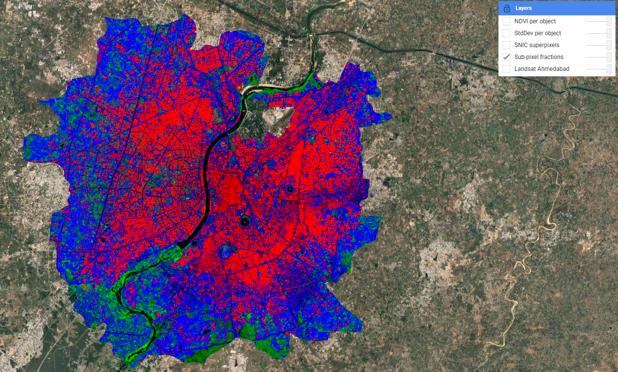
Spectral unmixing defines spectrally pure endmembers for each land cover class and computes the fractional contribution of each to every pixel. In GEE this is implemented via .unmix(), with constrained outputs ensuring fractions sum to 1. The result is a smooth, continuous surface — in contrast to the hard boundaries produced by Random Forest last week. The Sabarmati River appears as a clean black corridor, reflecting near-zero contributions from all non-water endmembers.
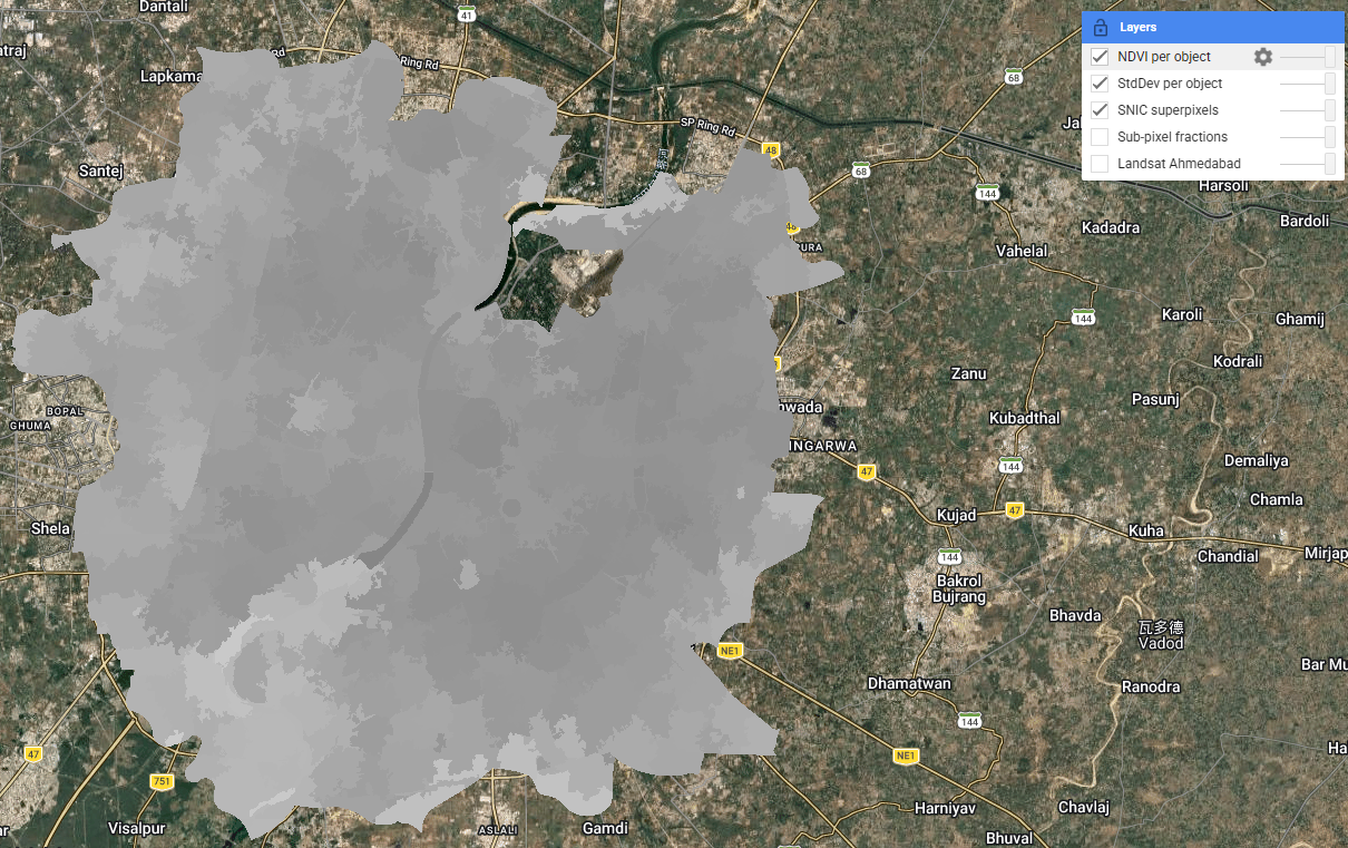
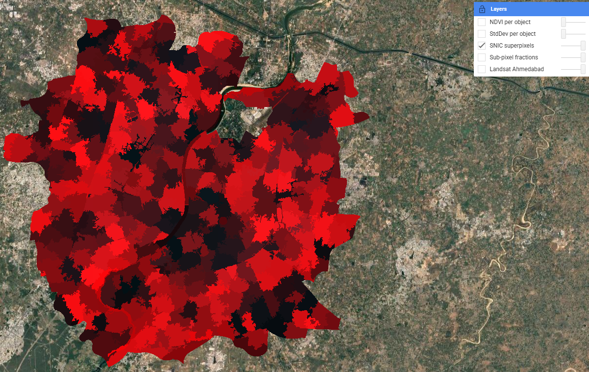
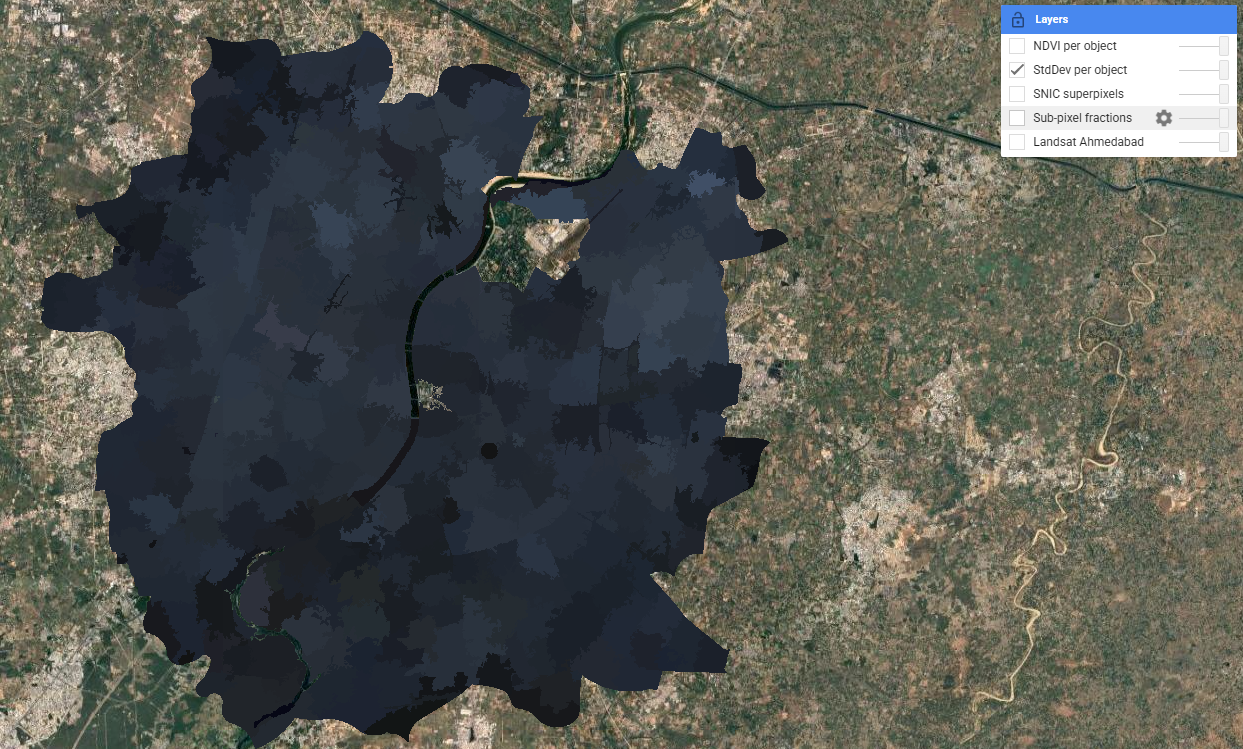
SNIC superpixels take a different approach: pixels are first grouped into spatially coherent objects based on spectral and spatial proximity, controlled by the compactness parameter. The resulting objects follow land cover boundaries far more naturally than a regular grid. Per-object NDVI and standard deviation were then computed as additional features — adding shape and texture context that pure spectral classification misses.
The lecture also covered accuracy assessment. The standard confusion matrix yields producer’s accuracy (TP/TP+FN), user’s accuracy (TP/TP+FP), and overall accuracy. The F1 score — harmonic mean of precision and recall — avoids optimising one at the expense of the other. The ROC curve and AUC show classifier performance across all decision thresholds; random guessing gives AUC = 0.5.
A critical warning from Karasiak et al. (2022) is that spatial autocorrelation between training and test pixels — when both are drawn from the same polygon — can massively inflate apparent accuracy. The solution is spatial cross-validation: partitioning sets using geographic distance to ensure spatial independence. The pixel-level split used in Week 6 partially addresses this but does not fully resolve the problem when training polygons are spatially clustered.
Applications
Sub-pixel and object-based methods have found particularly strong uptake in urban informal settlement mapping, where the heterogeneous mix of materials and the fine-grained spatial structure of slums makes pixel-based approaches unreliable. Matarira et al. (2023) combined Sentinel-1 SAR, Sentinel-2 optical and PlanetScope high-resolution data in an OBIA framework in GEE to map informal settlements in Durban, South Africa, achieving substantially better delineation of settlement boundaries than pixel-based methods. The ability of OBIA to incorporate shape, texture, and context — not just spectral values — is critical in this application: informal roofing materials often have similar spectral signatures to formal urban structures, but their spatial arrangement and object geometry differ markedly. This challenge also motivates deep learning approaches: Wurm et al. (2019) used fully convolutional neural networks on very high resolution imagery to segment slum areas, demonstrating that architectural and spatial patterns invisible to spectral classifiers can be learned directly from image structure.
The accuracy assessment issues raised in the lecture have direct implications for how classification results are used in policy. Karasiak et al. (2022) showed that spatial dependence between training and test data is a major source of overoptimistic accuracy — a problem particularly relevant for studies like urban heat island mapping in Ahmedabad, where training polygons are likely to be clustered in easily accessible or visually distinctive areas. If the reported accuracy of a green cover classification is inflated by spatial autocorrelation, and that classification is fed into the city’s Heat Action Plan to identify high-risk wards, the consequences of misclassification fall disproportionately on the most vulnerable communities. This connects accuracy assessment from a technical exercise to an ethical one. An alternative to custom classification is to use pre-classified products like Dynamic World (near real-time 10m Sentinel-2 based classification by Google), which uses a Fully Convolutional Neural Network trained on expert-labelled tiles — though as the lecture noted, its “blobby” appearance at boundaries reflects the 50×50m minimum mapping unit used in training.
Reflection
What I found most thought-provoking this week was the accuracy assessment discussion — specifically the point that spatial autocorrelation between training and test data can make a model look far more accurate than it actually is. Looking back at last week’s 88.7% overall accuracy, I have to acknowledge that because my training polygons were relatively small and clustered in recognisable areas of the city, the validation pixels drawn from those same polygons were almost certainly spatially correlated with the training pixels. A spatially cross-validated accuracy would likely be lower. This doesn’t invalidate the exercise, but it does mean I should treat the 88.7% figure as an upper bound rather than a reliable estimate. It’s a good reminder that accuracy metrics in remote sensing are not objective measurements — they reflect choices about how validation data is collected and structured, and those choices can be just as consequential as the classification algorithm itself.